Intragroup variance solution example. An example of finding the variance
Where σ 2 j is the intra-group variance of the j -th group.
For ungrouped data residual dispersion is a measure of the approximation accuracy, i.e. approximation of the regression line to the original data: 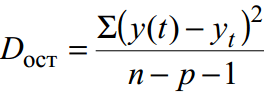
where y(t) is the forecast according to the trend equation; y t – initial series of dynamics; n is the number of points; p is the number of coefficients of the regression equation (the number of explanatory variables).
In this example it is called unbiased estimate of variance.
Example #1. The distribution of workers of three enterprises of one association by tariff categories is characterized by the following data:
| Worker's wage category | Number of workers at the enterprise | ||
| enterprise 1 | enterprise 2 | enterprise 3 | |
| 1 | 50 | 20 | 40 |
| 2 | 100 | 80 | 60 |
| 3 | 150 | 150 | 200 |
| 4 | 350 | 300 | 400 |
| 5 | 200 | 150 | 250 |
| 6 | 150 | 100 | 150 |
Define:
1. dispersion for each enterprise (intragroup dispersion);
2. average of intragroup dispersions;
3. intergroup dispersion;
4. total variance.
Solution.
Before proceeding to solve the problem, it is necessary to find out which feature is effective and which is factorial. In the example under consideration, the effective feature is "Tariff category", and the factor feature is "Number (name) of the enterprise".
Then we have three groups (enterprises) for which it is necessary to calculate the group average and intragroup variances:
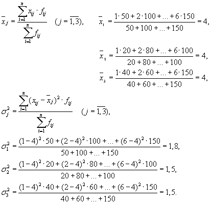
| Company | group average, | within-group variance, |
| 1 | 4 | 1,8 |
The average of the intragroup variances ( residual dispersion) calculated by the formula:

where you can calculate:
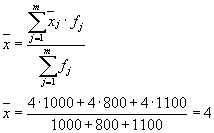
or:

Then:
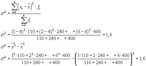
Total variance will be equal to: s 2 \u003d 1.6 + 0 \u003d 1.6.
The total variance can also be calculated using one of the following two formulas:
When solving practical problems, one often has to deal with a sign that takes only two alternative values. In this case, they are not talking about the weight of a particular value of a feature, but about its share in the aggregate. If the proportion of population units that have the trait under study is denoted by " R", and not possessing - through" q”, then the dispersion can be calculated by the formula:
s 2 = p×q
Example #2. According to the data on the development of six workers of the brigade, determine the intergroup variance and evaluate the impact of the work shift on their labor productivity if the total variance is 12.2.
| No. of the working brigade | Working output, pcs. | |
| in the first shift | in 2nd shift | |
| 1 | 18 | 13 |
| 2 | 19 | 14 |
| 3 | 22 | 15 |
| 4 | 20 | 17 |
| 5 | 24 | 16 |
| 6 | 23 | 15 |
Solution. Initial data
| X | f1 | f2 | f 3 | f4 | f5 | f6 | Total |
| 1 | 18 | 19 | 22 | 20 | 24 | 23 | 126 |
| 2 | 13 | 14 | 15 | 17 | 16 | 15 | 90 |
| Total | 31 | 33 | 37 | 37 | 40 | 38 |
Then we have 6 groups for which it is necessary to calculate the group mean and intragroup variances.
1. Find the average values of each group.
2. Find the mean square of each group.
We summarize the results of the calculation in a table:
| Group number | Group average | Intragroup variance |
| 1 | 1.42 | 0.24 |
| 2 | 1.42 | 0.24 |
| 3 | 1.41 | 0.24 |
| 4 | 1.46 | 0.25 |
| 5 | 1.4 | 0.24 |
| 6 | 1.39 | 0.24 |
3. Intragroup variance characterizes the change (variation) of the studied (resulting) trait within the group under the influence of all factors, except for the factor underlying the grouping:
We calculate the average of the intragroup dispersions using the formula:
4. Intergroup variance characterizes the change (variation) of the studied (resulting) trait under the influence of a factor (factorial trait) underlying the grouping.
Intergroup dispersion is defined as:
Where
Then
Total variance characterizes the change (variation) of the studied (resulting) trait under the influence of all factors (factorial traits) without exception. By the condition of the problem, it is equal to 12.2.
Empirical correlation relation measures how much of the total fluctuation of the resulting attribute is caused by the studied factor. This is the ratio of the factorial variance to the total variance:
We determine the empirical correlation relation:
Relationships between features can be weak or strong (close). Their criteria are evaluated on the Chaddock scale:
0.1 0.3 0.5 0.7 0.9 In our example, the relationship between feature Y factor X is weak
Determination coefficient.
Let's define the coefficient of determination:
Thus, 0.67% of the variation is due to differences between traits, and 99.37% is due to other factors.
Conclusion: in this case, the output of workers does not depend on work in a particular shift, i.e. the influence of the work shift on their labor productivity is not significant and is due to other factors.
Example #3. Based on average wages and squared deviations from its value for two groups of workers, find the total variance by applying the rule for adding variances:
Solution:Average of within-group variances
Intergroup dispersion is defined as:
The total variance will be: 480 + 13824 = 14304
 .
.
Conversely, if is a non-negative a.e. a function such that  , then there is an absolutely continuous probability measure on such that is its density.
Change of measure in the Lebesgue integral:
 ,
,
where is any Borel function integrable with respect to the probability measure .
Dispersion, types and properties of dispersion The concept of dispersion
Dispersion in statistics is found as the standard deviation of the individual values of the trait squared from the arithmetic mean. Depending on the initial data, it is determined by the simple and weighted variance formulas:
1. simple variance(for ungrouped data) is calculated by the formula:
![]()
2. Weighted variance (for a variation series):

where n - frequency (repeatability factor X)
An example of finding the variance
This page describes a standard example of finding the variance, you can also look at other tasks for finding it
Example 1. Determination of group, average of group, between-group and total variance
Example 2. Finding the variance and coefficient of variation in a grouping table
Example 3. Finding the variance in discrete series
Example 4. We have the following data for a group of 20 correspondence students. It is necessary to build an interval series of the feature distribution, calculate the mean value of the feature and study its variance

Let's build an interval grouping. Let's determine the range of the interval by the formula:
![]()
where X max is the maximum value of the grouping feature; X min is the minimum value of the grouping feature; n is the number of intervals:
We accept n=5. The step is: h \u003d (192 - 159) / 5 \u003d 6.6
Let's make an interval grouping

For further calculations, we will build an auxiliary table:

X "i - the middle of the interval. (for example, the middle of the interval 159 - 165.6 \u003d 162.3)
The average growth of students is determined by the formula of the arithmetic weighted average:

We determine the dispersion by the formula:
The formula can be converted like this:

From this formula it follows that the variance is the difference between the mean of the squares of the options and the square and the mean.
Dispersion in variation series With at equal intervals by the method of moments can be calculated in the following way using the second property of the dispersion (dividing all options by the value of the interval). Definition of variance, calculated by the method of moments, according to the following formula is less time consuming:

where i is the value of the interval; A - conditional zero, which is convenient to use the middle of the interval with the highest frequency; m1 is the square of the moment of the first order; m2 - moment of the second order
Feature variance (if in the statistical population the attribute changes in such a way that there are only two mutually exclusive options, then such variability is called alternative) can be calculated by the formula:

Substituting in this dispersion formula q = 1- p, we get:

Types of dispersion
Total variance measures the variation of a trait over the entire population as a whole under the influence of all the factors that cause this variation. It is equal to the mean square of the deviations of the individual values of the attribute x from the total average value x and can be defined as simple variance or weighted variance.
Intragroup variance characterizes random variation, i.e. part of the variation, which is due to the influence of unaccounted for factors and does not depend on the sign-factor underlying the grouping. This variance is equal to the mean square of the deviations of the individual values of the attribute within the X group from the arithmetic mean of the group and can be calculated as a simple variance or as a weighted variance.
Thus, within-group variance measures variation of a trait within a group and is determined by the formula:

where xi - group average; ni is the number of units in the group.
For example, intra-group variances, which must be determined in the task of studying the influence of workers' qualifications on the level of labor productivity in the shop, show variations in output in each group caused by all possible factors ( technical condition equipment, availability of tools and materials, age of workers, labor intensity, etc.), except for differences in the qualification category (within the group, all workers have the same qualifications).
The average of the within-group variances reflects random variation, that is, that part of the variation that occurred under the influence of all other factors, with the exception of the grouping factor. It is calculated by the formula:

Intergroup variance characterizes the systematic variation of the resulting trait, which is due to the influence of the trait-factor underlying the grouping. It is equal to the mean square of the deviations of the group means from the overall mean. Intergroup variance is calculated by the formula:

This page describes a standard example of finding the variance, you can also look at other tasks for finding it
Example 1. Determination of group, average of group, between-group and total variance
Example 2. Finding the variance and coefficient of variation in a grouping table
Example 3. Finding the variance in a discrete series
Example 4. We have the following data for a group of 20 correspondence students. It is necessary to build an interval series of the feature distribution, calculate the mean value of the feature and study its variance
Let's build an interval grouping. Let's determine the range of the interval by the formula:
![]()
where X max is the maximum value of the grouping feature;
X min is the minimum value of the grouping feature;
n is the number of intervals:
We accept n=5. The step is: h \u003d (192 - 159) / 5 \u003d 6.6
Let's make an interval grouping

For further calculations, we will build an auxiliary table:

X "i - the middle of the interval. (for example, the middle of the interval 159 - 165.6 \u003d 162.3)
The average growth of students is determined by the formula of the arithmetic weighted average:

We determine the dispersion by the formula:
The formula can be converted like this:

From this formula it follows that the variance is the difference between the mean of the squares of the options and the square and the mean.
Variance in variation series with equal intervals according to the method of moments can be calculated in the following way using the second dispersion property (dividing all options by the value of the interval). Definition of variance, calculated by the method of moments, according to the following formula is less time consuming:

where i is the value of the interval;
A - conditional zero, which is convenient to use the middle of the interval with the highest frequency;
m1 is the square of the moment of the first order;
m2 - moment of the second order
Feature variance (if in the statistical population the attribute changes in such a way that there are only two mutually exclusive options, then such variability is called alternative) can be calculated by the formula:

Substituting in this dispersion formula q = 1- p, we get:

Types of dispersion
Total variance measures the variation of a trait over the entire population as a whole under the influence of all the factors that cause this variation. It is equal to the mean square of the deviations of the individual values of the attribute x from the total average value x and can be defined as simple variance or weighted variance.
Intragroup variance characterizes random variation, i.e. part of the variation, which is due to the influence of unaccounted for factors and does not depend on the sign-factor underlying the grouping. This variance is equal to the mean square of the deviations of the individual values of the attribute within the X group from the arithmetic mean of the group and can be calculated as a simple variance or as a weighted variance.
Thus, within-group variance measures variation of a trait within a group and is determined by the formula:

where xi - group average;
ni is the number of units in the group.
For example, intra-group variances that need to be determined in the task of studying the effect of workers' qualifications on the level of labor productivity in a shop show variations in output in each group caused by all possible factors (technical condition of equipment, availability of tools and materials, age of workers, labor intensity, etc. .), except for differences in the qualification category (within the group, all workers have the same qualification).
Let's calculate inMSEXCELdispersion and standard deviation samples. We also calculate the variance random variable if its distribution is known.
First consider dispersion, then standard deviation.
Sample variance
Sample variance (sample variance,samplevariance) characterizes the spread of values in the array relative to .
All 3 formulas are mathematically equivalent.
It can be seen from the first formula that sample variance is the sum of the squared deviations of each value in the array from average divided by the sample size minus 1.
dispersion samples the DISP() function is used, eng. the name of the VAR, i.e. VARIance. Since MS EXCEL 2010, it is recommended to use its analogue DISP.V() , eng. the name VARS, i.e. Sample Variance. In addition, starting from the version of MS EXCEL 2010, there is a DISP.G () function, eng. VARP name, i.e. Population VARIance which calculates dispersion For population . The whole difference comes down to the denominator: instead of n-1 like DISP.V() , DISP.G() has just n in the denominator. Prior to MS EXCEL 2010, the VARP() function was used to calculate the population variance.
Sample variance
=SQUARE(Sample)/(COUNT(Sample)-1)
=(SUMSQ(Sample)-COUNT(Sample)*AVERAGE(Sample)^2)/ (COUNT(Sample)-1)- the usual formula
=SUM((Sample -AVERAGE(Sample))^2)/ (COUNT(Sample)-1) –
Sample variance is equal to 0 only if all values are equal to each other and, accordingly, are equal mean value. Usually, the larger the value dispersion, the greater the spread of values in the array.
Sample variance is point estimate dispersion distribution of the random variable from which the sample. About construction confidence intervals when evaluating dispersion can be read in the article.
Variance of a random variable
To calculate dispersion random variable, you need to know it.
For dispersion random variable X often use the notation Var(X). Dispersion is equal to the square of the deviation from the mean E(X): Var(X)=E[(X-E(X)) 2 ]
dispersion calculated by the formula:

where x i is the value that the random variable can take, and μ is the average value (), p(x) is the probability that the random variable will take the value x.
If the random variable has , then dispersion calculated by the formula:

Dimension dispersion corresponds to the square of the unit of measurement of the original values. For example, if the values in the sample are measurements of the weight of the part (in kg), then the dimension of the variance would be kg 2 . This can be difficult to interpret, therefore, to characterize the spread of values, a value equal to square root from dispersion – standard deviation.
Some properties dispersion:
Var(X+a)=Var(X), where X is a random variable and a is a constant.
Var(aХ)=a 2 Var(X)
Var(X)=E[(X-E(X)) 2 ]=E=E(X 2)-E(2*X*E(X))+(E(X)) 2=E(X 2)- 2*E(X)*E(X)+(E(X)) 2 =E(X 2)-(E(X)) 2
This dispersion property is used in article about linear regression.
Var(X+Y)=Var(X) + Var(Y) + 2*Cov(X;Y), where X and Y are random variables, Cov(X;Y) is the covariance of these random variables.
If random variables are independent, then their covariance is 0, and hence Var(X+Y)=Var(X)+Var(Y). This property of the variance is used in the output.
Let us show that for independent quantities Var(X-Y)=Var(X+Y). Indeed, Var(X-Y)= Var(X-Y)= Var(X+(-Y))= Var(X)+Var(-Y)= Var(X)+Var(-Y)= Var( X)+(-1) 2 Var(Y)= Var(X)+Var(Y)= Var(X+Y). This property of the variance is used to plot .
Sample standard deviation
Sample standard deviation is a measure of how widely scattered the values in the sample are relative to their .
A-priory, standard deviation equals the square root of dispersion:

Standard deviation does not take into account the magnitude of the values in sampling, but only the degree of scattering of values around them middle. Let's take an example to illustrate this.
Let's calculate the standard deviation for 2 samples: (1; 5; 9) and (1001; 1005; 1009). In both cases, s=4. It is obvious that the ratio of the standard deviation to the values of the array is significantly different for the samples. For such cases, use The coefficient of variation(Coefficient of Variation, CV) - ratio standard deviation to the average arithmetic, expressed as a percentage.
In MS EXCEL 2007 and earlier versions for calculation Sample standard deviation the function =STDEV() is used, eng. the name STDEV, i.e. standard deviation. Since MS EXCEL 2010, it is recommended to use its analogue = STDEV.B () , eng. name STDEV.S, i.e. Sample STandard DEViation.
In addition, starting from the version of MS EXCEL 2010, there is a function STDEV.G () , eng. name STDEV.P, i.e. Population STandard DEViation which calculates standard deviation For population. The whole difference comes down to the denominator: instead of n-1 like STDEV.V() , STDEV.G() has just n in the denominator.
Standard deviation can also be calculated directly from the formulas below (see example file)
=SQRT(SQUADROTIV(Sample)/(COUNT(Sample)-1))
=SQRT((SUMSQ(Sample)-COUNT(Sample)*AVERAGE(Sample)^2)/(COUNT(Sample)-1))
Other dispersion measures
The SQUADRIVE() function calculates with umm of squared deviations of values from their middle. This function will return the same result as the formula =VAR.G( Sample)*CHECK( Sample) , Where Sample- a reference to a range containing an array of sample values (). Calculations in the QUADROTIV() function are made according to the formula:

The SROOT() function is also a measure of the scatter of a set of data. The SIROTL() function calculates the average of the absolute values of the deviations of values from middle. This function will return the same result as the formula =SUMPRODUCT(ABS(Sample-AVERAGE(Sample)))/COUNT(Sample), Where Sample- a reference to a range containing an array of sample values.
Calculations in the function SROOTKL () are made according to the formula:

According to the sample survey, depositors were grouped according to the size of the deposit in the Sberbank of the city:
Define:
1) range of variation;
2) average deposit amount;
3) average linear deviation;
4) dispersion;
5) standard deviation;
6) coefficient of variation of contributions.
Solution:
This distribution series contains open intervals. In such series, the value of the interval of the first group is conventionally assumed to be equal to the value of the interval of the next, and the value of the interval of the last group is equal to the value of the interval of the previous one.
The interval value of the second group is 200, therefore, the value of the first group is also 200. The interval value of the penultimate group is 200, which means that the last interval will also have a value equal to 200.
1) Define the range of variation as the difference between the largest and the smallest value sign:
The range of variation in the size of the contribution is 1000 rubles.
2) The average size of the contribution is determined by the formula of the arithmetic weighted average.
Let's preliminarily define discrete quantity feature in each interval. To do this, using the simple arithmetic mean formula, we find the midpoints of the intervals.
The average value of the first interval will be equal to:

the second - 500, etc.
Let's put the results of calculations in the table:
| Deposit amount, rub. | Number of contributors, f | The middle of the interval, x | xf |
|---|---|---|---|
| 200-400 | 32 | 300 | 9600 |
| 400-600 | 56 | 500 | 28000 |
| 600-800 | 120 | 700 | 84000 |
| 800-1000 | 104 | 900 | 93600 |
| 1000-1200 | 88 | 1100 | 96800 |
| Total | 400 | - | 312000 |
The average deposit in the city's Sberbank will be 780 rubles:
3) The average linear deviation is the arithmetic average of the absolute deviations of the individual values of the attribute from the total average:

The procedure for calculating the average linear deviation in the interval distribution series is as follows:
1. The arithmetic weighted average is calculated, as shown in paragraph 2).
2. The absolute deviations of the variant from the mean are determined:
3. The obtained deviations are multiplied by the frequencies:
4. The sum of weighted deviations is found without taking into account the sign:
5. The sum of the weighted deviations is divided by the sum of the frequencies:
It is convenient to use the table of calculated data:
| Deposit amount, rub. | Number of contributors, f | The middle of the interval, x | |||
|---|---|---|---|---|---|
| 200-400 | 32 | 300 | -480 | 480 | 15360 |
| 400-600 | 56 | 500 | -280 | 280 | 15680 |
| 600-800 | 120 | 700 | -80 | 80 | 9600 |
| 800-1000 | 104 | 900 | 120 | 120 | 12480 |
| 1000-1200 | 88 | 1100 | 320 | 320 | 28160 |
| Total | 400 | - | - | - | 81280 |

The average linear deviation of the size of the deposit of Sberbank clients is 203.2 rubles.
4) Dispersion is the arithmetic mean of the squared deviations of each feature value from the arithmetic mean.
Calculation of dispersion in interval series distribution is made according to the formula:

The procedure for calculating the variance in this case is as follows:
1. Determine the arithmetic weighted average, as shown in paragraph 2).
2. Find deviations from the mean:
3. Squaring the deviation of each option from the mean:
4. Multiply squared deviations by weights (frequencies):
![]()
5. Summarize the received works:
![]()
6. The resulting amount is divided by the sum of the weights (frequencies):

Let's put the calculations in a table:
| Deposit amount, rub. | Number of contributors, f | The middle of the interval, x | |||
|---|---|---|---|---|---|
| 200-400 | 32 | 300 | -480 | 230400 | 7372800 |
| 400-600 | 56 | 500 | -280 | 78400 | 4390400 |
| 600-800 | 120 | 700 | -80 | 6400 | 768000 |
| 800-1000 | 104 | 900 | 120 | 14400 | 1497600 |
| 1000-1200 | 88 | 1100 | 320 | 102400 | 9011200 |
| Total | 400 | - | - | - | 23040000 |


