Forecasting based on the exponential smoothing method. Example of problem solution
How Forecast NOW! better model Exponential smoothing (ES) you can see in the graph below. The X axis is the product number, the Y axis is the percentage improvement in forecast quality. Read below for a description of the model, detailed research, and experimental results.
Model description
Forecasting method exponential smoothing is one of the most simple ways forecasting. The forecast can only be obtained for one period in advance. If forecasting is carried out in terms of days, then only one day ahead, if weeks, then one week.
For comparison, forecasting was carried out one week ahead for 8 weeks.
What is exponential smoothing?
Let the row WITH represents the original sales series for forecasting
C(1)- sales in the first week, WITH(2) in the second and so on.

Figure 1. Sales by week, row WITH
Likewise, the series S represents an exponentially smoothed sales series. The coefficient α ranges from zero to one. It turns out as follows, here t is a moment in time (day, week)
S (t+1) = S(t) + α *(С(t) - S(t))
Large values of the smoothing constant α speed up the response of the forecast to a jump in the observed process, but can lead to unpredictable outliers because there will be almost no smoothing.
For the first time after the start of observations, having only one observation result C (1) , when forecast S (1) no, and formula (1) cannot yet be used as a forecast S (2) should take C (1) .
The formula can easily be rewritten in a different form:
S (t+1) = (1 -α )* S (t)+α * WITH (t).
Thus, as the smoothing constant increases, the share of recent sales increases, and the share of smoothed previous sales decreases.
The constant α is selected experimentally. Typically, several forecasts are made for different constants and the most optimal constant is selected from the point of view of the selected criterion.
The criterion may be the accuracy of forecasting for previous periods.
In our study, we considered exponential smoothing models in which α takes values (0.2, 0.4, 0.6, 0.8). For comparison with the Forecast NOW! For each product, forecasts were made for each α, and the most accurate forecast was selected. In reality, the situation would be much more complicated; the user, without knowing in advance the accuracy of the forecast, needs to decide on the coefficient α, on which the quality of the forecast greatly depends. This is such a vicious circle.
Clearly

Figure 2. α =0.2, the degree of exponential smoothing is high, real sales are poorly taken into account

Figure 3. α =0.4, the degree of exponential smoothing is average, real sales are taken into account to an average degree
You can see how, as the constant α increases, the smoothed series increasingly corresponds to real sales, and if there are outliers or anomalies, we will get an extremely inaccurate forecast.

Figure 4. α =0.6, the degree of exponential smoothing is low, real sales are taken into account significantly
We can see that at α=0.8 the series almost exactly repeats the original one, which means the forecast tends to the rule “the same amount will be sold as yesterday”
It is worth noting that here it is absolutely impossible to focus on the error of approximation to the original data. You can achieve a perfect fit but still get an unacceptable prediction.

Figure 5. α =0.8, the degree of exponential smoothing is extremely low, real sales are taken into account heavily
Examples of forecasts
Now let's look at the predictions that are obtained using different meaningsα. As can be seen from Figures 6 and 7, the higher the smoothing coefficient, the more accurately the forecast repeats real sales with a one-step delay. Such a delay may in fact be critical, so you cannot simply choose the maximum value of α. Otherwise, we will get a situation where we say that exactly as much will be sold as was sold in the previous period.

Figure 6. Prediction of the exponential smoothing method at α=0.2

Figure 7. Prediction of the exponential smoothing method at α=0.6
Let's see what happens when α = 1.0. Let us recall that S is predicted (smoothed) sales, C is real sales.
S (t+1) = (1 -α )* S (t)+α * WITH (t).
S (t+1) = WITH (t).
Sales on day t+1 according to the forecast are equal to sales on the previous day. Therefore, the choice of constant must be approached wisely.
Comparison with Forecast NOW!
Now let's look at this forecasting method in comparison with Forecast NOW!. The comparison was made on 256 products that have different sales, with short-term and long-term seasonality, with “bad” sales and shortages, promotions and other outliers. For each product, a forecast was built using the exponential smoothing model, for different α, the best one was selected and compared with the forecast using the Forecast NOW! model.
In the table below you can see the forecast error value for each product. The error here was considered as RMSE. This is the root of standard deviation forecast from reality. Roughly speaking, it shows how many units of goods we deviated from the forecast. The improvement shows by what percentage the Forecast NOW! It is better if the number is positive, and worse if it is negative. In Figure 8, the X axis shows products, the Y axis indicates how much the Forecast NOW! better than forecasting using exponential smoothing. As you can see from this graph, the forecasting accuracy of Forecast NOW! almost always twice as high and almost never worse. What this means in effect is that using Forecast NOW! will allow you to halve inventories or reduce shortages.
Identifying and analyzing the trend of a time series is often done by flattening or smoothing it. Exponential smoothing is one of the simplest and most common methods for straightening a series. Exponential smoothing can be represented as a filter, the input of which is sequentially received from the terms of the original series, and the output is formed by the current values of the exponential average.
Let be a time series.
Exponential smoothing of the series is carried out using the recurrent formula: , .
The smaller α, the more the oscillations of the original series and noise are filtered and suppressed.
If we consistently use this recurrent relationship, then the exponential average can be expressed through the values of the time series X.
If earlier data exists when smoothing begins, then the arithmetic average of all available data or some part of it can be used as the initial value.
After the appearance of the works of R. Brown, exponential smoothing is often used to solve the problem of short-term forecasting of time series.
Formulation of the problem
Let the time series be given: .
It is necessary to solve the problem of forecasting a time series, i.e. find
Forecasting horizon, it is necessary that
In order to take into account data aging, we introduce a non-increasing sequence of weights, then
Brown model
Let us assume that D is small (short-term forecast), then to solve such a problem we use Brown model.
If we consider the forecast one step ahead, then the error of this forecast, and the new forecast is obtained as a result of adjusting the previous forecast taking into account its error - the essence of adaptation.
In short-term forecasting, it is desirable to reflect new changes as quickly as possible and at the same time “clean” the series from random fluctuations as best as possible. That. the weight of more recent observations should be increased: .
On the other hand, to smooth out random deviations, α needs to be reduced: .
That. these two requirements are in conflict. Finding a compromise value of α constitutes the model optimization problem. Typically, α is taken from the interval (0.1/3).
Examples

The work of exponential smoothing at α=0.2 on data from monthly reports on sales of foreign automobile brands in Russia for the period from January 2007 to October 2008. Let us note the sharp drops in January and February, when sales traditionally decline and rise at the beginning of summer.
Problems
The model only works for a short forecast horizon. Trend and seasonal changes are not taken into account. To take into account their influence, it is proposed to use the following models: Holt (linear trend is taken into account), Holt-Winters (multiplicative exponential trend and seasonality), Theil-Wage (additive linear trend and seasonality).
9 5. Exponential smoothing method. Selecting a smoothing constant
When using the method least squares to determine the forecast tendency (trend), it is assumed in advance that all retrospective data (observations) have the same information content. Obviously, it would be more logical to take into account the process of discounting the initial information, that is, the inequality of these data for developing a forecast. This is achieved in the exponential smoothing method by giving the latest observations of the time series (that is, the values immediately preceding the forecast lead period) more significant “weights” compared to the initial observations. The advantages of the exponential smoothing method also include the simplicity of computational operations and the flexibility of describing various process dynamics. The method has found the greatest application for the implementation of medium-term forecasts.
5.1. The essence of the exponential smoothing method
The essence of the method is that the time series is smoothed using a weighted “moving average”, in which the weights obey the exponential law. In other words, the further from the end of the time series the point for which the weighted moving average is calculated is, the less “participation it takes” in developing the forecast.
Let the original dynamic series consist of levels (series components) y t , t = 1 , 2 ,...,n . For each m successive levels of this series
(m dynamic series with a step equal to one. If m is an odd number, and it is preferable to take an odd number of levels, since in this case the calculated level value will be in the center of the smoothing interval and it can easily replace the actual value, then the following formula can be written to determine the moving average: t+ ξ t+ ξ ∑y i ∑y i i= t− ξ i= t− ξ 2ξ + 1 where y t is the moving average value for moment t (t = 1, 2,...,n); y i is the actual value of the level at moment i; i – serial number of the level in the smoothing interval. The value of ξ is determined from the duration of the smoothing interval. Because the m =2 ξ +1 for odd m, then ξ = m 2 − 1 . The calculation of a moving average with a large number of levels can be simplified by determining successive values of the moving average recursively: y t= y t− 1 + yt + ξ − y t − (ξ + 1 ) 2ξ + 1 But based on the fact that more “weight” needs to be given to recent observations, the moving average needs a different interpretation. It lies in the fact that the value obtained by averaging replaces not the central term of the averaging interval, but its last term. Accordingly, the last expression can be rewritten in the form Mi = Mi + 1 y i− y i− m Here the moving average referred to the end of the interval is indicated by the new symbol M i . Essentially, M i is equal to y t shifted ξ steps to the right, that is, M i = y t + ξ, where i = t + ξ. Considering that M i − 1 is an estimate of the quantity y i − m , expression (5.1) can be rewritten in the form y i+ 1 M i − 1 , M i , defined by expression (5.1). where M i is the estimate If calculations (5.2) are repeated as new information arrives and rewrite it in a different form, we obtain a smoothed observation function: Q i= α y i+ (1 − α ) Q i− 1 , or in equivalent form Q t= α y t+ (1 − α ) Q t− 1 Calculations carried out using expression (5.3) with each new observation are called exponential smoothing. In the last expression, to distinguish exponential smoothing from the moving average, the notation Q is introduced instead of M. The quantity α, which is analogue of m 1, is called the smoothing constant. The values of α lie in interval [0, 1]. If α is represented as a series α + α(1 − α) + α(1 − α) 2 + α(1 − α) 3 + ... + α(1 − α) n , then it is easy to notice that the “weights” decrease exponentially in time. For example, for α = 0, 2 we get 0,2 + 0,16 + 0,128 + 0,102 + 0,082 + … The sum of the series tends to unity, and the terms of the sum decrease with time. The value of Q t in expression (5.3) is the exponential average of the first order, that is, the average obtained directly from smoothing observation data (primary smoothing). Sometimes, when developing statistical models, it is useful to resort to the calculation of higher-order exponential averages, that is, averages obtained by repeated exponential smoothing. The general notation in recurrent form for exponential mean order k is: Q t (k)= α Q t (k− 1 )+ (1 − α ) Q t (− k1 ). The value of k varies within 1, 2, …, p,p+1, where p is the order of the forecast polynomial (linear, quadratic, and so on). Based on this formula for the exponential average of the first, second and third orders, the expressions are obtained Q t (1 )= α y t + (1 − α ) Q t (− 1 1 ); Q t (2 )= α Q t (1 )+ (1 − α ) Q t (− 2 1 ); Q t (3 )= α Q t (2 )+ (1 − α ) Q t (− 3 1 ). 5.2. Determining the parameters of the forecast model using the exponential smoothing method Obviously, to develop forecast values based on a time series using the exponential smoothing method, it is necessary to calculate the coefficients of the trend equation using exponential averages. The coefficient estimates are determined using the fundamental Brown-Meyer theorem, which connects the coefficients of the predictive polynomial with exponential averages of the corresponding orders: (−
1
) aˆ p α (1 − α )∞ −α
)
j (p − 1 + j ) ! ∑j p= 0 p! (k− 1 ) !j = 0 where aˆ p are estimates of the coefficients of the degree polynomial. The coefficients are found by solving the system of (p + 1) equations сp + 1 unknown. So, for the linear model aˆ 0 = 2 Q t (1 ) − Q t (2 ) ; aˆ 1 = 1 − α α (Q t (1 )− Q t (2 )) ; for quadratic model aˆ 0 = 3 (Q t (1 )− Q t (2 )) + Q t (3 ); aˆ 1 =1 − α α [ (6 −5 α ) Q t (1 ) −2 (5 −4 α ) Q t (2 ) +(4 −3 α ) Q t (3 ) ] ; aˆ 2 = (1 − α α ) 2 [ Q t (1 )− 2 Q t (2 )+ Q t (3 )] . The forecast is implemented using the selected polynomial, respectively, for the linear model ˆyt + τ = aˆ0 + aˆ1 τ ; for quadratic model ˆyt + τ = aˆ0 + aˆ1 τ + aˆ 2 2 τ 2 , where τ is the prediction step. It should be noted that exponential averages Q t (k) can be calculated only with a known (selected) parameter, knowing the initial conditions Q 0 (k). Estimates of initial conditions, in particular for a linear model Q(1)=a 1 − α Q(2 ) = a− 2 (1 − α ) a for quadratic model Q(1)=a 1 − α + (1 − α )(2 − α ) a 2(1− α ) (1− α )(3− 2α ) Q 0(2 ) = a 0− 2α 2 Q(3)=a 3(1− α ) (1 − α )(4 − 3 α ) a where the coefficients a 0 and a 1 are calculated using the least squares method. The value of the smoothing parameter α is approximately calculated by the formula α ≈ m 2 + 1, where m is the number of observations (values) in the smoothing interval. The sequence of calculating forecast values is presented in Calculation of series coefficients using the least squares method Defining the smoothing interval Calculation of the smoothing constant Calculation of initial conditions Calculating exponential averages Calculation of estimates a 0 , a 1 , etc. Calculation of forecast values of a series Rice. 5.1. Sequence of calculation of predicted values As an example, consider the procedure for obtaining the predicted value of failure-free operation of a product, expressed by mean time between failures. The initial data are summarized in table. 5.1. We choose a linear forecasting model in the form y t = a 0 + a 1 τ The solution is feasible with the following values of the initial quantities: a 0, 0 = 64, 2; a 1, 0 = 31, 5; α = 0.305. Table 5.1. Initial data Observation number, t Step length, prediction, τ MTBF, y (hour) With these values, the calculated “smoothed” coefficients for the values of y 2 will be equal = α Q (1)− Q (2)= 97, 9; [ Q (1 )− Q (2 ) 31,
9 , 1− α at initial conditions 1 − α A 0 , 0 − a 1, 0 = −7
,
6
1 − α = −79
,
4
and exponential averages Q (1 )= α y + (1 − α ) Q (1 ) 25,
2;
Q(2) = α Q (1) + (1 −α ) Q (2 ) = −47 . 5 . The “smoothed” value y 2 is calculated using the formula Qi(1) Qi(2) a 0 ,i a 1 ,i ˆyt Thus (Table 5.2), the linear forecast model has the form ˆy t + τ = 224.5+ 32τ . Let's calculate the forecast values for lead times of 2 years (τ = 1), 4 years (τ = 2) and so on between product failures (Table 5.3). Table 5.3. Forecast valuesˆy t The equation t+2 t+4 t+6 t+8 t+20 regression (τ = 1) (τ = 2) (τ = 3) (τ = 5) τ =
ˆy t = 224.5+ 32τ It should be noted that the total “weight” of the last m values of the time series can be calculated using the formula c = 1 − (m (− 1 ) m ) . m+ 1 So, for the last two observations of the series (m = 2), the value c = 1 − (2 2 − + 1 1) 2 = 0.667. 5.3. Selecting initial conditions and determining the smoothing constant As follows from the expression Q t= α y t+ (1 − α ) Q t− 1 , When performing exponential smoothing, it is necessary to know the initial (previous) value of the smoothed function. In some cases, the first observation can be taken as the initial value; more often, the initial conditions are determined according to expressions (5.4) and (5.5). In this case, the values a 0, 0,a 1, 0 and a 2 , 0 are determined by the least squares method. If we do not have much confidence in the chosen initial value, then by taking a large value of the smoothing constant α through k observations we will get “weight” of the initial value to the value (1 − α ) k<<
α
, и оно будет практически забыто. Наоборот, если мы уверены в правильности выбранного начального значения и неизменности модели в течение определенного отрезка времени в будущем,α
может быть выбрано малым (близким к 0). Thus, choosing a smoothing constant (or the number of observations in a moving average) involves making a trade-off decision. Typically, as practice shows, the value of the smoothing constant lies in the range from 0.01 to 0.3. Several transitions are known that allow one to find an approximate estimate of α. The first follows from the condition of equality of the moving and exponential averages α = m 2 + 1, where m is the number of observations in the smoothing interval. Other approaches are associated with forecast accuracy. Thus, it is possible to determine α based on the Meyer relation: α ≈ S y, where S y – root mean square error of the model; S 1 – root mean square error of the original series. However, the use of the latter relationship is complicated by the fact that it is very difficult to reliably determine S y and S 1 from the initial information. Often the smoothing parameter, and at the same time the coefficients a 0, 0 and a 0, 1 are selected optimal depending on the criterion S 2 = α ∑ ∞ (1 − α ) j [ yij − ˆyij ] 2 → min j= 0 by solving an algebraic system of equations, which is obtained by equating the derivatives to zero ∂S2 ∂S2 ∂S2 ∂a 0, 0 ∂a 1, 0 ∂a 2, 0 Thus, for a linear forecasting model, the initial criterion is equal to S 2 = α ∑ ∞ (1 − α ) j [ yij − a0 , 0 − a1 , 0 τ ] 2 → min. j= 0 Solving this system using a computer does not present any difficulties. To make a reasonable choice of α, you can also use the generalized smoothing procedure, which allows you to obtain the following relations connecting the forecast variance and the smoothing parameter for the linear model: S p 2 ≈[ 1 + α β ] 2 [ 1 +4 β +5 β 2 +2 α (1 +3 β ) τ +2 α 2 τ 3 ] S y 2 for quadratic model S p 2≈ [ 2 α + 3 α 3+ 3 α 2τ ] S y 2, where β =
1
−
α
;Sy– RMS deviation of the approximation of the original time series. Forecasting problems are based on changes in certain data over time (sales, demand, supplies, GDP, carbon emissions, population...) and projecting these changes into the future. Unfortunately, trends identified from historical data can be disrupted by many unforeseen circumstances. So data in the future may differ significantly from what happened in the past. This is the problem of forecasting. However, there are techniques (called exponential smoothing) that allow you to not only try to predict the future, but also quantify the uncertainty of everything associated with the forecast. Numerically expressing uncertainty through the creation of forecast intervals is truly invaluable, but often overlooked in the forecasting world. Download the note in or format, examples in format Let’s say you are a fan of “The Lord of the Rings” and have been making and selling swords for three years now (Fig. 1). Let's display sales graphically (Fig. 2). Demand has doubled in three years - maybe this is a trend? We'll come back to this idea a little later. The graph has several peaks and valleys, which may be a sign of seasonality. Specifically, the peaks occur in months numbered 12, 24 and 36, which happen to be December. But maybe this is just a coincidence? Let's find out. Exponential smoothing methods rely on predicting the future from data from the past, where newer observations weigh more heavily than older ones. This weighting is possible thanks to smoothing constants. The first exponential smoothing method we'll try is called simple exponential smoothing (SES). It uses only one smoothing constant. Simple exponential smoothing assumes that your time series data consists of two components: a level (or average) and some error around that value. There is no trend or seasonal fluctuation - there is simply a level around which demand fluctuates, surrounded by small errors here and there. By giving preference to newer observations, TEC may cause shifts in this level. In the language of formulas, Demand at time t = level + random error around the level at time t So how do you find the approximate level value? If we accept all time values as having the same value, then we should simply calculate their average value. However, this is a bad idea. More weight should be given to recent observations. Let's create several levels. Let's calculate the initial level in the first year: level 0 = average demand for the first year (months 1-12) For the demand for swords it is 163. We use level 0 (163) as the demand forecast for month 1. Demand for month 1 is 165, that is, it is 2 swords above level 0. It is worth updating the baseline approximation. The equation for simple exponential smoothing is: level 1 = level 0 + a few percent × (demand 1 – level 0) level 2 = level 1 + a few percent × (demand 2 – level 1) Etc. “A few percent” is called the smoothing constant, and is denoted by alpha. This can be any number from 0 to 100% (0 to 1). You will learn how to choose the alpha value later. In general, the value for different times is: Level current period = level previous period + Future demand is equal to the last calculated level (Fig. 3). Since you don't know what alpha is, set cell C2 to 0.5 to start with. After the model is built, find an alpha such that the sum of squared error - E2 (or standard deviation - F2) is minimal. To do this, run the option Finding a solution. To do this, go through the menu DATA –> Finding a solution, and install in the window Solution Search Options required values (Fig. 4). To display the forecast results on a chart, first select the range A6:B41 and build a simple line chart. Next, right-click on the diagram and select the option Select data. In the window that opens, create a second row and insert predictions from the range A42:B53 into it (Fig. 5). To test this assumption, it is enough to fit a linear regression to the demand data and perform a t test on the rise of this trend line (as in). If the slope of the line is non-zero and statistically significant (in testing using the Student’s t-test, the value R less than 0.05), the data has a trend (Fig. 6). We used the LINEST function, which returns 10 descriptive statistics (if you have not used this function before, I recommend it) and the INDEX function, which allows you to “pull out” only the three required statistics, and not the entire set. It turned out that the slope is 2.54, and it is significant, since the Student's test showed that 0.000000012 is significantly less than 0.05. So, there is a trend, and all that remains is to include it in the forecast. It is often called double exponential smoothing because it has not one smoothing parameter - alpha, but two. If a time sequence has a linear trend, then: demand for time t = level + t × trend + random level deviation at time t Holt Exponential Smoothing with Trend Adjustment has two new equations, one for the level as it moves through time, and the other for the trend. The level equation contains a smoothing parameter alpha, and the trend equation contains gamma. Here's what the new level equation looks like: level 1 = level 0 + trend 0 + alpha × (demand 1 – (level 0 + trend 0)) note that level 0 + trend 0 is just a one-step forecast from initial values to month 1, so demand 1 – (level 0 + trend 0)- this is a one-step deviation. Thus, the basic level approximation equation will be: level current period = level previous period + trend previous period + alpha × (demand current period – (level previous period) + trend previous period)) Trend update equation: trend current period = trend previous period + gamma × alpha × (demand current period – (level previous period) + trend previous period)) Holt smoothing in Excel is similar to simple smoothing (Figure 7), and as above, the goal is to find two coefficients while minimizing the sum of squared errors (Figure 8). To get the initial level and trend values (in cells C5 and D5 in Figure 7), plot a graph for the first 18 months of sales and add a trend line with an equation to it. Enter the initial trend value of 0.8369 and the initial level of 155.88 in cells C5 and D5. Forecast data can be presented graphically (Fig. 9). Rice. 7. Holt exponential smoothing with trend adjustment; To enlarge the image, right-click on it and select Open image in new tab There is a way to test the strength of a predictive model - compare the errors with themselves, shifted by a step (or several steps). If the deviations are random, then the model cannot be improved. However, there may be a seasonal factor in the demand data. The concept of an error term that is correlated with another period's version of itself is called autocorrelation (for more on autocorrelation, see ). To calculate autocorrelation, start with forecast error data for each period (column F in Figure 7 moves to column B in Figure 10). Next, determine the average forecast error (Fig. 10, cell B39; formula in cell: =AVERAGE(B3:B38)). In column C, calculate the deviation of the forecast error from the mean; formula in cell C3: =B3-B$39. Next, sequentially shift column C one column to the right and a row down. Formulas in cells D39: =SUMPRODUCT($C3:$C38,D3:D38), D41: =D39/$C39, D42: =2/SQRT(36), D43: =-2/SQRT(36). What does it mean for one of the D:O columns to be “synchronous” with column C? For example, if columns C and D are synchronous, then a number that is negative in one of them must be negative in the other, positive in one, positive in friend. This means that the sum of the products of the two columns will be significant (the differences accumulate). Or, which is the same, the closer the value in the range D41:O41 is to zero, the lower the correlation of the column (from D to O, respectively) with column C (Fig. 11). One autocorrelation is above the critical value. The error shifted by a year correlates with itself. This means a 12 month seasonal cycle. And this is not surprising. If you look at the demand graph (Fig. 2), it turns out that there are peaks in demand every Christmas and troughs in April-May. Let's consider a forecasting technique that takes into account seasonality. The method is called multiplicative (from multiplicate - multiply), because it uses multiplication to take into account seasonality: Demand at time t = (level + t × trend) × seasonal adjustment for time t × any remaining irregular adjustments that we cannot account for Holt-Winters smoothing is also called triple exponential smoothing because it has three smoothing parameters (alpha, gamma, and delta). For example, if there is a 12 month seasonal cycle: Forecast for month 39 = (level 36 + 3 × trend 36) x seasonality 27 When analyzing data, it is necessary to find out what is a trend in a data series and what is seasonality. To perform calculations using the Holt-Winters method, you must: Start with the raw data (columns A and B in Figure 12) and add column C with the moving average smoothed values. Since seasonality has 12-month cycles, it makes sense to use a 12-month average. There is a slight problem with this average. 12 is an even number. If you smooth out month 7 demand, should you consider it to be the average demand from months 1 to 12 or from months 2 to 13? To overcome this difficulty, you need to smooth out demand using a “2x12 moving average.” That is, take half of the two averages from months 1 to 12 and from months 2 to 13. The formula in cell C8: =(AVERAGE(B3:B14)+AVERAGE(B2:B13))/2. Smoothed data for months 1–6 and 31–36 cannot be obtained, since there are not enough previous and subsequent periods. For clarity, the original and smoothed data can be reflected in the diagram (Fig. 13). Now in column D, divide the original value by the smoothed one and get the approximate seasonal adjustment value (column D in Fig. 12). The formula in cell D8 is =B8/C8. Note the spikes of 20% above normal demand in months 12 and 24 (December), while troughs are observed in the spring. This smoothing technique gave you two point estimates for each month (24 months total). Column E finds the average of these two factors. Formula in cell E1: =AVERAGE(D14,D26). For clarity, the level of seasonal fluctuations can be presented graphically (Fig. 14). Seasonally adjusted data can now be obtained. The formula in cell G1 is: =B2/E2. Construct a graph based on the data in column G, supplement it with a trend line, display the trend equation on the chart (Fig. 15), and use the coefficients in subsequent calculations. Form a new sheet as shown in Fig. 16. Substitute the values in the range E5:E16 from Fig. 12 areas E2:E13. Take the values of C16 and D16 from the trend line equation in Fig. 15. Set the values of the smoothing constants to start at 0.5. Stretch the values in line 17 to cover the range of months 1 through 36. Run Finding a solution to optimize smoothing coefficients (Fig. 18). The formula in cell B53 is: =(C$52+(A53-A$52)*D$52)*E41. Now you need to check the autocorrelations in the forecast made (Fig. 18). Since all the values are located between the upper and lower boundaries, you understand that the model has done a good job of understanding the structure of demand values. So, we have a completely working forecast. How do you set upper and lower bounds that can be used to make realistic assumptions? The Monte Carlo simulation that you have already encountered in (see also) will help you with this. The idea is to generate future scenarios of demand behavior and identify the group in which 95% of them fall. Remove the forecast from cells B53:B64 from the Excel sheet (see Fig. 17). You will record the demand there based on the simulation. The latter can be generated using the NORMINV function. For future months, you just need to supply it with the mean (0), the standard distribution (10.37 from cell $H$2) and a random number between 0 and 1. The function will return the deviation with a probability corresponding to a bell curve. Place the one-step error simulation in cell G53: =NORMIN(RAND(),0,H$2). Stretch this formula down to G64 and you get forecast error simulations for 12 months of a one-step forecast (Figure 19). Your simulation values will differ from those shown in the figure (that’s why it’s a simulation!). With forecast uncertainty, you have everything you need to update the level, trend and seasonal coefficient. So select cells C52:F52 and stretch them to row 64. As a result, you have a simulated forecast error and the forecast itself. Based on the opposite, we can predict demand values. Insert the formula into cell B53: =F53+G53 and stretch it to B64 (Fig. 20, range B53:F64). Now you can press the F9 button, updating the forecast each time. Place the results of 1000 simulations in cells A71:L1070, each time transposing the values from the range B53:B64 to the range A71:L71, A72:L72, ... A1070:L1070. If this bothers you, write some VBA code. Now you have 1000 scenarios for each month, and you can use the PERCENTILE function to get the upper and lower bounds at the middle of the 95% confidence interval. In cell A66 the formula is: =PERCENTILE(A71:A1070,0.975), and in cell A67: =PERCENTILE(A71:A1070,0.025). As usual, for clarity, the data can be presented graphically (Fig. 21). There are two interesting points in the graph: Written based on the book by John Foreman. – M.: Alpina Publisher, 2016. – P. 329–381 The development of new and analysis of known management technologies that can improve the efficiency of business management is becoming especially relevant for Russian enterprises at the present time. One of the most popular tools is the budgeting system, which is based on the formation of an enterprise budget with subsequent monitoring of execution. The budget represents balanced short-term commercial, production, financial and economic plans for the development of the organization. The enterprise budget contains targets that are calculated based on forecast data. The most significant forecast when drawing up a budget for any business is the sales forecast. In previous articles, an analysis of the additive and multiplicative model was carried out and the forecast sales volume for the following periods was calculated. When analyzing time series, the moving average method was used, in which all data, regardless of the period of their occurrence, are equal. There is another way in which weights are assigned to data, with more recent data being given more weight than earlier data. The exponential smoothing method, unlike the moving average method, can also be used for short-term forecasts of future trends one period in advance and automatically adjusts any forecast in light of differences between the actual and predicted results. That is why the method has a clear advantage over the previously discussed one. The name of the method comes from the fact that it produces exponentially weighted moving averages over the entire time series. With exponential smoothing, all previous observations are taken into account - the previous one is taken into account with maximum weight, the one preceding it with slightly less weight, the earliest observation affects the result with minimal statistical weight. The algorithm for calculating exponentially smoothed values at any point in the series i is based on three quantities: actual value of Ai at a given point in series i, The new forecast can be written as: Calculation of exponentially smoothed values
When using the exponential smoothing method in practice, two problems arise: the choice of the smoothing coefficient (W), which significantly affects the results, and the determination of the initial condition (Fi). On the one hand, to smooth out random deviations, the value must be reduced. On the other hand, to increase the weight of new dimensions, it is necessary to increase. Although, in principle, W can take any value from the range 0< W < 1, обычно ограничиваются интервалом от 0,2 до 0,5. При высоких значениях коэффициента сглаживания в большей степени учитываются мгновенные текущие наблюдения отклика (для динамично развивающихся фирм) и, наоборот, при низких его значениях сглаженная величина определяется в большей степени прошлой тенденцией развития, нежели текущим состоянием отклика системы (в условиях стабильного развития рынка). The choice of smoothing constant is subjective. Analysts at most companies use their traditional values of W when processing series. Thus, according to published data in the analytical department of Kodak, they traditionally use a value of 0.38, and at Ford Motors - 0.28 or 0.3. Manual calculation of exponential smoothing requires an extremely large amount of monotonous work. Using the example, we will calculate the forecast volume for the 13th quarter, if sales data are available for the last 12 quarters, using the simple exponential smoothing method. Let's assume that the sales forecast for the first quarter was 3. And let the smoothing coefficient W = 0.8. Let's fill in the third column in the table, substituting for each subsequent quarter the value of the previous one using the formula: For 2nd quarter F2 =0.8*4 (1-0.8)*3 =3.8 Similarly, the smoothed value is calculated for the coefficient 0.5 and 0.33. The forecast for sales volume with W = 0.8 for the 13th quarter amounted to 13.3 thousand rubles. This data can be presented in graphical form:


Initial data

Simple exponential smoothing
alpha × (demand current period – level previous period)


Perhaps you have a trend

Holt Exponential Smoothing with Trend Adjustment


Identifying patterns in data


Holt-Winters multiplicative exponential smoothing


Constructing a confidence interval for the forecast


Ph.D., Director for Science and Development of JSC "KIS"
Exponential smoothing method
forecast at a point in the series Fi
some predetermined smoothing coefficient W, constant over the entire series.
For the 3rd quarter F3 =0.8*6 (1-0.8)*3.8 =5.6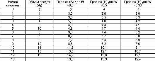
Calculation of sales volume forecast

Exponential smoothing