Construct discrete and interval distribution series. Construction of a discrete variational series

27.09.2019 | Internet

What is the grouping of statistical data, and how it is related to the distribution series, was considered in this lecture, where you can also learn about what a discrete and variational distribution series is.

The distribution series is one of the varieties statistical series(besides them, time series are used in statistics), are used to analyze data on phenomena public life. The construction of variational series is quite a feasible task for everyone. However, there are rules to remember.

How to build a discrete variational distribution series

Example 1 Data are available on the number of children in 20 surveyed families. Construct a discrete variational series distribution of families by number of children.

0 1 2 3 1
2 1 2 1 0
4 3 2 1 1
1 0 1 0 2

Solution:

Let's start with the layout of the table, in which we will then enter the data. Since the distribution rows have two elements, the table will consist of two columns. The first column is always a variant - what we are studying - we take its name from the task (the end of the sentence with the task in the conditions) - by number of children- so our version is the number of children.

The second column is the frequency - how often our variant occurs in the phenomenon under study - we also take the name of the column from the task - distribution of families - so our frequency is the number of families with the corresponding number of children.

Now, from the initial data, we select those values that occur at least once. In our case, this

And let's arrange this data in the first column of our table in a logical order, in this case increasing from 0 to 4. We get

And in conclusion, let's calculate how many times each value of the options occurs.

0 1 2 3 1

2 1 2 1 0

4 3 2 1 1

1 0 1 0 2

As a result, we obtain a complete table or the required series of distribution of families by the number of children.

Exercise . There is data on the tariff categories of 30 workers of the enterprise. Construct a discrete variational series for the distribution of workers by wage category. 2 3 2 4 4 5 5 4 6 3

1 4 4 5 5 6 4 3 2 3

4 5 4 5 5 6 6 3 3 4

How to build an interval variation series of distribution

Let's build interval series distribution, and let's see how its construction differs from a discrete series.

Example 2 There is data on the amount of profit received by 16 enterprises, million rubles. — 23 48 57 12 118 9 16 22 27 48 56 87 45 98 88 63. at equal intervals.

The general principle of constructing a series, of course, will be preserved, the same two columns, the same variants and frequency, but in this case the variants will be located in the interval and the frequencies will be counted differently.

Solution:

Let's start similarly to the previous task by building a table layout, into which we will then enter data. Since the distribution rows have two elements, the table will consist of two columns. The first column is always a variant - what we are studying - we take its name from the task (the end of the sentence with the task in the conditions) - by the amount of profit - which means that our variant is the amount of profit received.

The second column is the frequency - how often our variant occurs in the phenomenon under study - we also take the name of the column from the assignment - the distribution of enterprises - this means our frequency is the number of enterprises with the corresponding profit, in this case falling into the interval.

As a result, the layout of our table will look like this:

where i is the value or length of the interval,

Xmax and Xmin - the maximum and minimum value of the feature,

n is the required number of groups according to the condition of the problem.

Let's calculate the interval value for our example. To do this, among the initial data, we find the largest and smallest

23 48 57 12 118 9 16 22 27 48 56 87 45 98 88 63 - the maximum value is 118 million rubles, and the minimum is 9 million rubles. Let's calculate the formula.

In the calculation, we got the number 36, (3) three in the period, in such situations, the value of the interval must be rounded up so that after the calculations the maximum data is not lost, which is why the value of the interval in the calculation is 36.4 million rubles.

Now let's build the intervals - our options in this problem. The first interval is started from the minimum value, the value of the interval is added to it and the upper limit of the first interval is obtained. Then the upper limit of the first interval becomes the lower limit of the second interval, the value of the interval is added to it and the second interval is obtained. And so on as many times as required to build intervals according to the condition.

Pay attention, if we did not round the value of the interval to 36.4, but would leave it at 36.3, then the last value would be 117.9. It is in order to avoid data loss that it is necessary to round the value of the interval to a larger value.

Let's count the number of enterprises that fall into each specific interval. When processing data, it must be remembered that the upper value of the interval in this interval is not taken into account (is not included in this interval), but is taken into account in the next interval (the lower limit of the interval is included in this interval, and the upper one is not included), except for the last interval.

When carrying out data processing, it is best to indicate the selected data with conventional icons or color to simplify processing.

23 48 57 12 118 9 16 22

27 48 56 87 45 98 88 63

We will mark the first interval in yellow - and determine how much data falls into the interval from 9 to 45.4, while this 45.4 will be taken into account in the second interval (provided that it is in the data) - as a result, we get 7 enterprises in the first interval. And so on for all intervals.

(additional action) Let's calculate the total amount of profit received by enterprises for each interval and in general. To do this, we add the data marked different colors and get the total value of profit.

For the first interval 23 + 12 + 9 + 16 + 22 + 27 + 45 = 154 million rubles

For the second interval - 48 + 57 + 48 + 56 + 63 = 272 million rubles.

For the third interval - 118 + 87 + 98 + 88 = 391 million rubles.

Exercise . There is data on the size of the deposit in the bank of 30 depositors, thousand rubles. 150, 120, 300, 650, 1500, 900, 450, 500, 380, 440,

600, 80, 150, 180, 250, 350, 90, 470, 1100, 800,

500, 520, 480, 630, 650, 670, 220, 140, 680, 320

Build interval variation series distribution of depositors, by the size of the contribution, highlighting 4 groups at equal intervals. For each group, calculate the total amount of contributions.

Statistical distribution series- this is an ordered distribution of population units into groups according to a certain varying attribute.
Depending on the trait underlying the formation of a distribution series, there are attribute and variation distribution series.

The presence of a common feature is the basis for the formation of a statistical population, which is the results of a description or measurement common features research objects.

The subject of study in statistics are changing (variable) features or statistical features.

Types of statistical features.

Distribution series are called attribute series. built on quality grounds. Attributive- this is a sign that has a name (for example, a profession: a seamstress, teacher, etc.).
It is customary to arrange the distribution series in the form of tables. In table. 2.8 shows an attribute series of distribution.
Table 2.8 - Distribution of types of legal assistance provided by lawyers to citizens of one of the regions of the Russian Federation.

Variation series are feature values (or ranges of values) and their frequencies.
Variation series are distribution series built on a quantitative basis. Any variational series consists of two elements: variants and frequencies.
Variants are individual values of a feature that it takes in a variation series.
Frequencies are the numbers of individual variants or each group variation series, i.e. these are numbers showing how often certain options occur in a distribution series. The sum of all frequencies determines the size of the entire population, its volume.
Frequencies are called frequencies, expressed in fractions of a unit or as a percentage of the total. Accordingly, the sum of the frequencies is equal to 1 or 100%. The variational series allows us to evaluate the form of the distribution law based on actual data.

Depending on the nature of the variation of the trait, there are discrete and interval variation series.
An example of a discrete variational series is given in Table. 2.9.
Table 2.9 - Distribution of families by the number of rooms occupied in individual apartments in 1989 in the Russian Federation.

The first column of the table presents variants of a discrete variational series, the second column contains the frequencies of the variational series, and the third column contains the frequency indicators.

Variation series

IN population some quantitative trait is being investigated. A sample of volume is randomly extracted from it n, that is, the number of elements in the sample is n. At the first stage of statistical processing, ranging samples, i.e. number ordering x 1 , x 2 , …, x n Ascending. Each observed value x i called option. Frequency m i is the number of observations of the value x i in the sample. Relative frequency (frequency) w i is the frequency ratio m i to sample size n: .
When studying a variational series, the concepts of cumulative frequency and cumulative frequency are also used. Let x some number. Then the number of options , whose values are less x, is called the accumulated frequency: for x i n is called the accumulated frequency w i max .
An attribute is called discretely variable if its individual values (variants) differ from each other by some finite amount (usually an integer). A variational series of such a feature is called a discrete variational series.

Table 1. General view of the discrete variational series of frequencies

Feature values	x i	x 1	x2	…	x n
Frequencies	m i	m 1	m2	…	m n

An attribute is called continuously varying if its values differ from each other by an arbitrarily small amount, i.e. the sign can take any value in a certain interval. A continuous variation series for such a trait is called an interval series.

Table 2. General view of the interval variation series of frequencies

Table 3. Graphic images of the variation series

Row	Polygon or histogram	Empirical distribution function
Discrete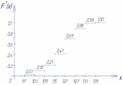
interval

Looking at the results of the observations, it is determined how many values of the options fell into each specific interval. It is assumed that each interval belongs to one of its ends: either in all cases the left (more often), or in all cases the right, and the frequencies or frequencies show the number of options contained in the indicated boundaries. Differences a i – a i +1 are called partial intervals. To simplify subsequent calculations, the interval variation series can be replaced by a conditionally discrete one. In this case, the mean value i-th interval is taken as an option x i, and the corresponding interval frequency m i- for the frequency of this interval.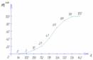
For graphic representation of variational series, polygon, histogram, cumulative curve and empirical distribution function are most often used.

In table. 2.3 (Grouping of the population of Russia according to the size of the average per capita income in April 1994) is presented interval variation series.
It is convenient to analyze the distribution series using a graphical representation, which also makes it possible to judge the shape of the distribution. A visual representation of the nature of the change in the frequencies of the variational series is given by polygon and histogram.
The polygon is used when displaying discrete variational series.
Let us depict, for example, graphically the distribution of housing stock by type of apartments (Table 2.10).
Table 2.10 - Distribution of the housing stock of the urban area by type of apartments (conditional figures).

Rice. Housing distribution polygon

On the y-axis, not only the values of frequencies, but also the frequencies of the variation series can be plotted.
The histogram is taken to display the interval variation series. When constructing a histogram, the values of the intervals are plotted on the abscissa axis, and the frequencies are depicted by rectangles built on the corresponding intervals. The height of the columns in the case of equal intervals should be proportional to the frequencies. A histogram is a graph in which a series is shown as bars adjacent to each other.
Let's graphically depict the interval distribution series given in Table. 2.11.
Table 2.11 - Distribution of families by the size of living space per person (conditional figures).

N p / p	Groups of families by the size of living space per person	Number of families with a given size of living space	Accumulated number of families
1	3 – 5	10	10
2	5 – 7	20	30
3	7 – 9	40	70
4	9 – 11	30	100
5	11 – 13	15	115
TOTAL		115	----

Rice. 2.2. Histogram of the distribution of families by the size of living space per person

Using the data of the accumulated series (Table 2.11), we construct distribution cumulative.

Rice. 2.3. The cumulative distribution of families by the size of living space per person

The representation of a variational series in the form of a cumulate is especially effective for variational series, the frequencies of which are expressed as fractions or percentages of the sum of the frequencies of the series.
If we change the axes in the graphic representation of the variational series in the form of a cumulate, then we get ogivu. On fig. 2.4 shows an ogive built on the basis of the data in Table. 2.11.
A histogram can be converted to a distribution polygon by finding the midpoints of the sides of the rectangles and then connecting these points with straight lines. The resulting distribution polygon is shown in fig. 2.2 dotted line.
When constructing a histogram of the distribution of a variational series with unequal intervals, along the ordinate axis, not frequencies are applied, but the distribution density of the feature in the corresponding intervals.
The distribution density is the frequency calculated per unit interval width, i.e. how many units in each group are per unit interval value. An example of calculating the distribution density is presented in Table. 2.12.
Table 2.12 - Distribution of enterprises by the number of employees (figures are conditional)

N p / p	Groups of enterprises by the number of employees, pers.	Number of enterprises	Interval size, pers.	Distribution density
	A	1	2	3=1/2
1	up to 20	15	20	0,75
2	20 – 80	27	60	0,25
3	80 – 150	35	70	0,5
4	150 – 300	60	150	0,4
5	300 – 500	10	200	0,05
	TOTAL	147	----	----

For a graphical representation of variation series can also be used cumulative curve. With the help of the cumulate (the curve of the sums), a series of accumulated frequencies is displayed. Accumulated frequencies are determined by sequentially summing the frequencies by groups and show how many units of the population have feature values no greater than the considered value.

Rice. 2.4. Ogiva distribution of families according to the size of living space per person

When constructing the cumulate of an interval variation series, the variants of the series are plotted along the abscissa axis, and the accumulated frequencies along the ordinate axis.

The characteristics studied by statistics vary (differ from each other) for different units of the population in the same period or point in time. For example, the value of foreign trade turnover varies by division of the FCS; the value of exports (imports) varies by direction of export (for different partner countries in foreign trade), by types of goods, etc.

Cause variations are different conditions for the existence of different units of the population. For example, a huge number of reasons affect the scale of foreign trade of various countries of the world.

To control and study variation by statistics, special methods for studying variation have been developed, a system of indicators by which variation is measured and its properties are characterized.

The first step in the statistical study of variation is the construction distribution series(or variation series) - ordered distribution of units of the population according to increasing (more often) or decreasing (less often) values of the attribute and counting the number of units with one or another value of the attribute.

There are 3 kind distribution range:

1) ranked row- this is a list of individual units of the population in ascending order of the trait under study (for example, table 11); if the number of population units is large enough, the ranked series becomes cumbersome, and in such cases, the distribution series is constructed by grouping the population units according to the values of the trait under study (if the trait takes a small number of values, then a discrete series is built, and otherwise, an interval series);

2) discrete series- this is a table consisting of two columns (rows) - specific values \u200b\u200bof a varying attribute Xi and the number of population units with the given value of the feature fi– frequencies; the number of groups in a discrete series is determined by the number of actually existing values of the variable attribute;

3) interval series- this is a table consisting of two columns (rows) - intervals of a varying sign Xi and the number of population units falling within a given interval (frequencies), or the proportion of this number in the total number of populations (frequencies).

Let's build a distribution series of foreign trade turnover (TO) by customs posts in Russia, for which it is necessary to carry out statistical observation, that is, to collect primary statistical material, which is the value of VO by customs posts.

The results of the observation of VO at 35 customs posts of the region for the reporting period will be presented in the form of a distribution series ranked in ascending order of the value of VO (Table 11).

Table 11. Foreign trade turnover (VO) for 35 customs posts, mln.

post number	post number	post number

Let us determine the average size of the VO according to the formula (10), taking for X the value of VO, and for N- number of posts:

= = 2100/35 = 60 (million dollars)

The variance (it will be discussed a little later - at the 4th stage of the analysis of variation in this topic) is determined by the formula (28):

= = 445.778 (million dollars2)

Let's build an interval series of VO distribution by customs posts, for which it is necessary to choose the optimal number of groups (character intervals) and set the length (range) of the interval. Since when analyzing a distribution series, frequencies are compared in different intervals, it is necessary that the length of the intervals be constant. The optimal number of groups is chosen so that the diversity of the trait values in the aggregate is sufficiently reflected and at the same time the regularity of the distribution, its shape is not distorted by random frequency fluctuations. If there are too few groups, there will be no pattern of variation; if there are too many groups, random frequency jumps will distort the shape of the distribution.

Most often, the number of groups in the distribution series is determined by the Sturgess formula (19) or (20):

(19) or ,(20)

Where k– number of groups (rounded to the nearest whole number); N- the size of the population.

It can be seen from the Sturgess formula that the number of groups is a function of the amount of data ( N).

Knowing the number of groups, the length (range) of the interval is calculated using the formula (21):

,(21)

Where X max and X min - the maximum and minimum values in the aggregate.

In our example about VO, using the Sturgess formula (19), we determine the number of groups:

k = 1 + 3,322lg 35 = 1+ 3,322*1,544 = 6,129 ≈ 6.

Calculate the length (range) of the interval using formula (21):

h= (111.16 - 24.16)/6 = 87/6 = 14.5 (million dollars).

Now let's build an interval series with 6 groups with an interval of 14.5 million dollars. (see the first 3 columns of Table 12).

Table 12. Interval series of VO distribution by customs posts, mln.

Groups of posts by the size of VO	Number of posts	Interval midpoint	X i' fi	Accum. frequency	\| Xi’ - \|fi	(Xi’ - )2 fi	(Xi’ - )3 fi	(Xi’ - )4 fi





96,66 – 111,16

A graphical representation provides essential assistance in the analysis of a distribution series and its properties. The interval series is represented by a bar graph, in which the bases of the bars, located along the abscissa axis, are the intervals of values of the varying attribute, and the heights of the bars are the frequencies corresponding to the scale along the ordinate axis. A graphic representation of the distribution of customs posts in the sample by the value of VO is shown in fig. 4. This type of diagram is called histogram .

Rice. 4. Distribution histogram 5. Distribution polygon

Table data. 12 and fig. 4 show the form of distribution characteristic of many traits: the values of the average intervals of the trait are more common, and the extreme (small and large) values of the trait are less common. The form of this distribution is close to the normal distribution law, which is formed if a variable variable is influenced by a large number of factors, none of which has a predominant value.

If there is a discrete distribution series or the midpoints of the intervals are used (as in our example about VO - in Table 12 in the 4th column the midpoints of the intervals are calculated as a half-sum of the values of the beginning and end of the interval), then the graphical representation of such a series is called polygon(see Fig. 5) , which is obtained by connecting straight points with coordinates Xi And fi.

In many cases, if the statistical population includes a large or, even more so, an infinite number of options, which is most often encountered with continuous variation, it is practically impossible and impractical to form a group of units for each option. In such cases, the association of statistical units into groups is possible only on the basis of the interval, i.e. such a group that has certain limits of the values of the varying attribute. These limits are indicated by two numbers indicating the upper and lower limits of each group. The use of intervals leads to the formation of an interval distribution series.

interval rad is a variational series, the variants of which are presented as intervals.

The interval series can be formed with equal and unequal intervals, while the choice of the principle for constructing this series depends mainly on the degree of representativeness and convenience of the statistical population. If the set is sufficiently large (representative) in terms of the number of units and is quite homogeneous in composition, then it is advisable to base the formation of the interval series on equal intervals. Usually, according to this principle, an interval series is formed for those populations where the range of variation is relatively small, i.e. the maximum and minimum variants usually differ from each other by several times. In this case, the value of equal intervals is calculated by the ratio of the range of the trait variation to the given number of formed intervals. To determine equal And interval, the Sturgess formula can be used (usually with a small variation in interval features and a large number of units in the statistical population):

where x i - the value of an equal interval; X max, X min - maximum and minimum options in the statistical population; n . - the number of units in the population.

Example. It is advisable to calculate the size of an equal interval according to the density of radioactive contamination with cesium - 137 in 100 settlements of the Krasnopolsky district of the Mogilev region, if it is known that the initial (minimum) variant is equal to I km / km 2, the final ( maximum) - 65 ki / km 2. Using the formula 5.1. we get:

Therefore, in order to form an interval series with equal intervals for the density of cesium pollution - 137 settlements of the Krasnopolsky district, the size of an equal interval can be 8 ki/km 2 .

In conditions of uneven distribution i.e. when the maximum and minimum options are hundreds of times, when forming the interval series, you can apply the principle unequal intervals. Unequal intervals usually increase as you move to larger values of the feature.

The shape of the intervals can be closed and open. Closed It is customary to name intervals for which both the lower and upper boundaries are indicated. open intervals have only one boundary: in the first interval - the upper, in the last - the lower boundary.

It is advisable to evaluate interval series, especially those with unequal intervals, taking into account distribution density, the simplest way to calculate which is the ratio of the local frequency (or frequency) to the size of the interval.

For the practical formation of the interval series, you can use the layout of the table. 5.3.

T a b l e 5.3. The procedure for the formation of an interval series of settlements in the Krasnopolsky district according to the density of radioactive contamination with cesium -137

The main advantage of the interval series is its limit compactness. at the same time, in the interval series of the distribution, the individual variants of the trait are hidden in the corresponding intervals

When a graphical representation of an interval series in a system of rectangular coordinates, the upper boundaries of the intervals are plotted on the abscissa axis, and the local frequencies of the series are on the ordinate axis. The graphical construction of an interval series differs from the construction of a distribution polygon in that each interval has a lower and an upper boundary, and two abscissas correspond to any value of the ordinate. Therefore, on the graph of the interval series, not a point is marked, as in a polygon, but a line connecting two points. These horizontal lines are connected to each other by vertical lines and a figure of a stepped polygon is obtained, which is commonly called histogram distributions (Figure 5.3).

In the graphical construction of an interval series for a sufficiently large statistical population, the histogram approaches symmetrical distribution form. In those cases where the statistical population is small, as a rule, it is formed asymmetric bar chart.

In some cases, there is expediency in the formation of a number of accumulated frequencies, i.e. cumulative row. A cumulative series can be formed on the basis of a discrete or interval distribution series. When a cumulative series is graphically displayed in a system of rectangular coordinates, options are plotted on the abscissa axis, and accumulated frequencies (frequencies) are plotted on the ordinate axis. The resulting curved line is called cumulative distributions (Figure 5.4).

The formation and graphical representation of various types of variational series contributes to a simplified calculation of the main statistical characteristics, which are discussed in detail in topic 6, helps to better understand the essence of the laws of distribution of a statistical population. The analysis of the variation series is of particular importance in cases where it is necessary to identify and trace the relationship between variants and frequencies (frequencies). This dependence is manifested in the fact that the number of cases for each variant is in a certain way related to the value of this variant, i.e. with an increase in the values of the varying sign of the frequency (frequency) of these values, they experience certain, systematic changes. This means that the numbers in the column of frequencies (frequencies) are not subject to chaotic fluctuations, but change in a certain direction, in a certain order and sequence.

If the frequencies in their changes show a certain systematicity, then this means that we are on the way to identifying patterns. The system, order, sequence in changing frequencies is a reflection of common causes, general conditions that are characteristic of the entire population.

It should not be assumed that the pattern of distribution is always given ready-made. There are quite a lot of variational series in which the frequencies bizarrely jump, either increasing or decreasing. In such cases, it is advisable to find out what kind of distribution the researcher is dealing with: either this distribution is not inherent in patterns at all, or its nature has not yet been identified: The first case is rare, while the second, the second case is a rather frequent and very common phenomenon.

So, when forming an interval series, the total number of statistical units can be small, and a small number of options fall into each interval (for example, 1-3 units). In such cases, it is not necessary to count on the manifestation of any regularity. In order for a regular result to be obtained on the basis of random observations, the law of large numbers must come into force, i.e. so that for each interval there would be not several, but tens and hundreds of statistical units. To this end, we must try to increase the number of observations as much as possible. This is the surest way to detect patterns in mass processes. If there is no real opportunity to increase the number of observations, then the identification of patterns can be achieved by reducing the number of intervals in the distribution series. Reducing the number of intervals in the variation series, thereby increasing the number of frequencies in each interval. This means that the random fluctuations of each statistical unit are superimposed on each other, "smoothed out", turning into a pattern.

The formation and construction of variational series allows you to get only a general, approximate picture of the distribution of the statistical population. For example, a histogram only roughly expresses the relationship between the values of a feature and its frequencies (frequencies). Therefore, variational series are essentially only the basis for further, in-depth study of the internal patterns of static distribution.

TOPIC 5 QUESTIONS

1. What is variation? What causes the variation of a trait in a statistical population?

2. What types of variable signs can take place in statistics?

3. What is a variation series? What are the types of variation series?

4. What is a ranked series? What are its advantages and disadvantages?

5. What is a discrete series and what are its advantages and disadvantages?

6. What is the order of formation of the interval series, what are its advantages and disadvantages?

7. What is a graphical representation of a ranked, discrete, interval distribution series?

8. What is distribution cumulate and what does it characterize?

Higher professional education

"RUSSIAN ACADEMY OF PEOPLE'S ECONOMY AND

CIVIL SERVICE UNDER THE PRESIDENT

RUSSIAN FEDERATION"

(Kaluga branch)

Department of Natural Science and Mathematical Disciplines

TEST

Subject "Statistics"

Student ___ Mayboroda Galina Yurievna ______

Correspondence department faculty State and municipal management group G-12-V

Lecturer ____________________ Hamer G.V.

PhD, Associate Professor

Kaluga-2013

Task 1.

Task 1.1. 4

Task 1.2. 16

Task 1.3. 24

Task 1.4. 33

Task 2.

Task 2.1. 43

Task 2.2. 48

Task 2.3. 53

Task 2.4. 58

Task 3.

Task 3.1. 63

Task 3.2. 68

Task 3.3. 73

Task 3.4. 79

Task 4.

Problem 4.1. 85

Task 4.2. 88

Task 4.3. 90

Task 4.4. 93

List of used sources. 96

Task 1.

Task 1.1.

There are the following data on the output and the amount of profit by the enterprises of the region (table 1).

Table 1

Data on the output and the amount of profits by enterprises

company number	Output, million rubles	Profit, million rubles	company number	Output, million rubles	Profit, million rubles
	63,0	6,7		56,0	7,2
	48,0	6,2		81,0	9,6
	39,0	6,5		55,0	6,3
	28,0	3,0		76,0	9,1
	72,0	8,2		54,0	6,0
	61,0	7,6		53,0	6,4
	47,0	5,9		68,0	8,5
	37,0	4,2		52,0	6,5
	25,0	2,8		44,0	5,0
	60,0	7,9		51,0	6,4
	46,0	5,5		50,0	5,8
	34,0	3,8		65,0	6,7
	21,0	2,1		49,0	6,1
	58,0	8,0		42,0	4,8
	45,0	5,7		32,0	4,6

According to the original data:

1. Build a statistical series of distribution of enterprises by output, forming five groups at equal intervals.

Build distribution series graphs: polygon, histogram, cumulate. Graphically determine the value of mode and median.

2. Calculate the characteristics of a series of distribution of enterprises by output: arithmetic mean, dispersion, standard deviation, coefficient of variation.

Make a conclusion.

3. Using the method of analytical grouping, establish the presence and nature of the correlation between the cost of manufactured products and the amount of profit per enterprise.

4. Measure the tightness of the correlation between the cost of production and the amount of profit by the empirical correlation.

Draw general conclusions.

Solution:

Let's build a statistical series of distribution

To construct an interval variation series that characterizes the distribution of enterprises in terms of output, it is necessary to calculate the value and boundaries of the intervals of the series.

When constructing a series with equal intervals, the value of the interval h is determined by the formula:

x max And x min- the largest and smallest values of the attribute in the studied set of enterprises;

k- number of interval series groups.

Number of groups k specified in the assignment. k= 5.

x max= 81 million rubles, x min= 21 million rubles

Calculation of the interval value:

million rubles

By successively adding the value of the interval h = 12 million rubles. to the lower boundary of the interval, we obtain the following groups:

1 group: 21 - 33 million rubles.

2 group: 33 - 45 million rubles;

Group 3: 45 - 57 million rubles.

Group 4: 57 - 69 million rubles.

Group 5: 69 - 81 million rubles.

To construct an interval series, it is necessary to calculate the number of enterprises included in each group ( group frequencies).

The process of grouping enterprises by output volume is presented in auxiliary table 2. Column 4 of this table is necessary to build an analytical grouping (item 3 of the task).

table 2

Table for constructing an interval distribution series and

analytical grouping

Groups of enterprises by output, million rubles	company number	Output, million rubles	Profit, million rubles
21-33		21,0	2,1
	25,0	2,8
	28,0	3,0
	32,0	4,6
Total		106,0	12,5
33-45		34,0	3,8
	37,0	4,2
	39,0	6,5
	42,0	4,8
	44,0	5,0
Total		196,0	24,3
45-57		45,0	5,7
	46,0	5,5
	47,0	5,9
	48,0	6,2
	49,0	6,1
	50,0	5,8
	51,0	6,4
	52,0	6,5
	53,0	6,4
	54,0	6,0
	55,0	6,3
	56,0	7,2
Total		606,0	74,0
57-69		58,0	8,0
	60,0	7,9
	61,0	7,6
	63,0	6,7
	65,0	6,7
	68,0	8,5
Total		375,0	45,4
69-81		72,0	8,2
	76,0	9,1
	81,0	9,6
Total		229,0	26,9
Total			183,1

Based on the group summary rows of the "Total" table 3, a final table 3 is formed, representing the interval series of the distribution of enterprises by output.

Table 3

A number of distribution of enterprises by output volume

Conclusion. The constructed grouping shows that the distribution of enterprises in terms of output is not uniform. The most common enterprises with a production volume of 45 to 57 million rubles. (12 enterprises). The least common are enterprises with output from 69 to 81 million rubles. (3 enterprises).

Let's build graphs of the distribution series.

Polygon often used to represent discrete series. To construct a polygon in a rectangular coordinate system, the values of the argument are plotted on the abscissa axis, i.e. options (for interval variation series, the middle of the interval is taken as an argument) and on the ordinate axis - frequency values. Further, in this coordinate system, points are built, the coordinates of which are pairs of corresponding numbers from the variation series. The resulting points are connected in series by straight line segments. The polygon is shown in Figure 1.

bar chart - bar chart. It allows you to evaluate the symmetry of the distribution. The histogram is shown in Figure 2.

Figure 1 - Polygon distribution of enterprises by volume

output

Fashion

Figure 2 - Histogram of the distribution of enterprises by volume

output

Fashion- the value of the trait that occurs most often in the study population.

For an interval series, the mode can be graphically determined from the histogram (Figure 2). For this, the highest rectangle is selected, which in this case is modal (45–57 million rubles). Then the right vertex of the modal rectangle is connected to the upper right corner of the previous rectangle. And the left vertex of the modal rectangle is with the upper left corner of the subsequent rectangle. Further, from the point of their intersection, a perpendicular is lowered to the abscissa axis. The abscissa of the point of intersection of these lines will be the distribution mode.

Million rub.

Conclusion. In the considered set of enterprises, the most common are enterprises with a product output of 52 million rubles.

Cumulate - broken curve. It is built on the accumulated frequencies (calculated in Table 4). The cumulate starts from the lower boundary of the first interval (21 million rubles), the accumulated frequency is deposited at the upper boundary of the interval. The cumulate is shown in Figure 3.

Median

Figure 3 - Cumulative distribution of enterprises by volume

output

Median Me is the value of the feature that falls in the middle of the ranked series. There are the same number of population units on both sides of the median.

In an interval series, the median can be determined graphically from a cumulative curve. To determine the median from a point on the cumulative frequency scale corresponding to 50% (30:2 = 15), a straight line is drawn parallel to the abscissa axis until it intersects with the cumulate. Then, from the point of intersection of the specified straight line with the cumulate, a perpendicular is lowered to the abscissa axis. The abscissa of the intersection point is the median.

Million rub.

Conclusion. In the considered set of enterprises, half of the enterprises have a production volume of no more than 52 million rubles, and the other half - no less than 52 million rubles.

Similar information.